Noisy Elo II
This post follows the Noisy Elo post from over 4 years ago(!) which in turns follows How good is Elo for predicting chess?. Let’s do a bit of recap:
Recap
In How good is Elo for predicting chess?, we observed that the Elo formula systematically overpredicts the expected score of the better player. For example, if one player has an Elo rating that’s 400 above their opponent, the Elo formula predicts an average score of 0.91 (which you can very approximately interpret as a 91% chance of winning), however empirically that player only averages a score of about 0.85 (using a dataset of about 10 million online games played on https://lichess.org).
In Noisy Elo, we made a guess at what might explain the underperformance of actual expected scores relative to the Elo formula’s prediction: maybe Elo ratings are a noisy measurement of true Elo ratings. We assumed that the noise was normally distributed with zero mean, and we fit a standard deviation empirically. It turned out a standard deviation of 110 fit the data well.
We left off by musing about what could give us more confidence in our guess that noise is what explains why the Elo formula overpredicts the expected score of the better player. This situation felt reminiscent of progress in physics:
You have a theory for how the world works, but new empirical data shows up that disagrees with the theory. Assuming the new data is valid, you try to come up with a new model that fits the data. And you find one! Your model fits the new data well. But how do you convince others to use your new model, especially in light of potentially other new models that also fit the data? One approach is to propose a new experiment for which your model predicts a different outcome than the old model. If your model predicts the correct outcome of a yet-to-be-conducted experiment, for which the old model would have been wrong, that’s fairly compelling evidence to start using it in place of the old model.
The experiment
Here’s the intuition for the experiment: All the Elo formula cares about is the difference of the two ratings. It doesn’t matter whether the two players have ratings of (1500 and 1900) or (2500 and 2900) – both pairs of ratings have a difference of 400 and so the Elo formula will predict the same score for the better player in both scenarios.
Our model might not have that property. Intuitively, I’d expect our model to predict a lower score for the 2900 player in the 2500 vs. 2900 game than the 1900 player in the 1500 vs. 1900 game. Why? Because our model won’t “believe” the 2500 or 2900 ratings as much as the 1500 and 1900 ratings because they’re so rare. It will assume a lot of the 2500 and 2900 rating is noise. I’m expecting our model to “squeeze” the 2500 and 2900 ratings closer together than the 1500 and 1900 ratings when predicting the true Elos. If that’s right, then the expected score of the 2900 player will be closer to 0.5 (an even match) than the expected score of the 1900 player.
If our model makes different predictions than the tweaked Elo formula that we fit to empirical data, it provides an opportunity to test our theory. We can see whether empirical results depend on the absolute ratings or just the difference between ratings. If empirical results depend on absolute ratings, that suggests our theory might be correct.
Let’s see!
The plan: I want to compute the expected score of a 1900 rated player when playing a 1500 rated player. Likewise for a 2900 rated player when playing a 2500 rated player.
Assumptions: We’re going to assume that “true Elo” is normally distributed with a mean of 1630 and a stdev of 290. Rating are a noisy measurement of true Elo, with noise $\mathcal{N}(0, 110)$ (fit empirically in the last post), which makes ratings $\mathcal{N}(1630, 310)$ (also fit empirically).
As a step towards computing the expected score of a 1900 rated player when playing a 1500 rated player, let me first compute the expected true Elo of a 1900 rated player. In fact, why don’t I just compute it for all possible ratings:
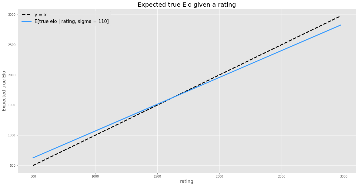
Huh! That looks… more like a line than I expected. I added the line $y=x$ to help see that the slope of E[true Elo | rating] is less than 1. In other words, we tend to expect true Elos to be closer to the population average (1630) than their rating. That part definitely makes sense.
But I didn’t expect it to be a straight line. Remember, I expected our model to squeeze 2500 and 2900 ratings closer together than 1500 and 1900. But that’s not what this line is telling me. The fact that it’s a line means it will squeeze them by exactly the same amount. Let’s demonstrate that:
| Rating | Expected true Elo |
|---|---|
| 1500 | 1514.5 |
| 1900 | 1869.8 |
| 2500 | 2402.7 |
| 2900 | 2758.0 |
The expected difference in true Elo between the 1500 and 1900 rated players is (1869.8 - 1514.5) = 355.3 and the expected difference in true Elo between the 2500 and 2900 rated players is (2758 - 2402.7) = 355.3. The same!
So my intuition was wrong. The expected difference in true Elo between two players does not depend on their absolute ratings, only the difference between their ratings. The experiment failed before it even began…
A silver lining
Well, the experiment failed, but maybe there’s a silver lining. Recall that the elo formula predicts a score of 0.91 for the better player when the rating difference is 400, but we found that empirically the rating difference needed to be more like 525 in order for the expected score of the better player to be 0.91. Maybe we have a simple explanation for this. Maybe we need the rating difference to be 525 because then the expected true Elo difference is 400. Let’s check.
| Rating | Expected true Elo |
|---|---|
| 1500 | 1514.5 |
| 2025 | 1980.8 |
The difference in the expected true Elo is (1980.8 - 1514.5) = 466. Huh! Wrong again.
An instructive mistake
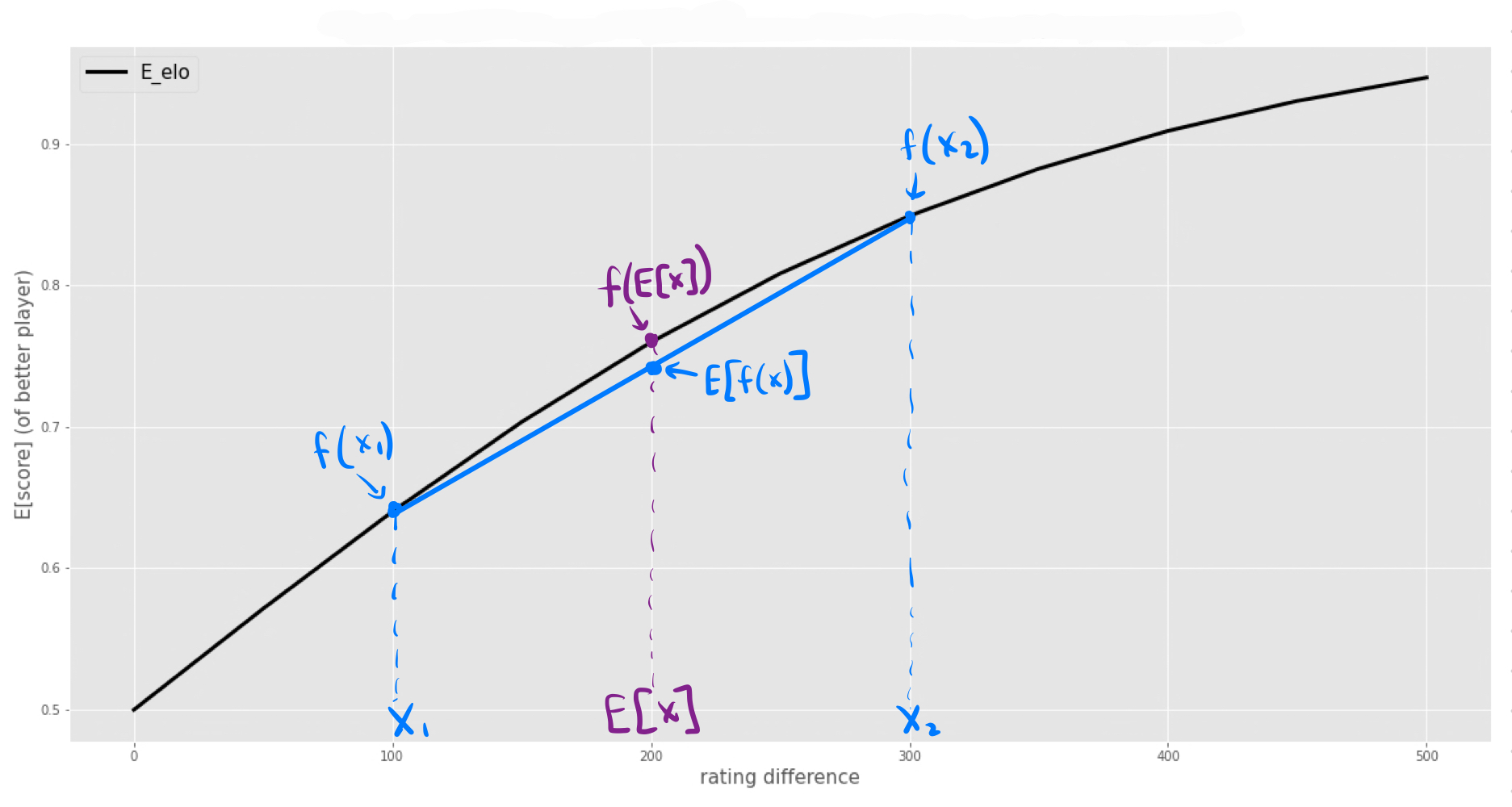
I made a classic mistake (and I honestly did make this mistake) - did you spot it? I assumed that EloFormula(E[true Elo difference]) = E[EloFormula(true Elo difference)]. I computed the former by plugging in the expected true Elo difference into the formula, but what we really want to compute is the expected value of formula given all the possible true Elo differences (weighted by their probability).
For concave functions like the Elo formula $E[f(x)] < f(E[x])$. I can show you why on the graph:
Computing the expected score correctly
What we need to do is first compute E[f(x)] – not f(E[x]). To do that, let’s first find the PDF of the true Elo difference given a rating difference of 525, and then use that entire distribution to compute the expected score of the better player (by plugging in those true Elo differences into the Elo formula and taking a weighed average of the results).
How can we compute the PDF of the true Elo difference given a rating difference of 525?
A long digression about normal distributions
Here’s a fact about adding two normal distributions that we’ve used before:
\[\begin{align} X &\sim \mathcal{N}( \mu_x,\sigma_x) \\ Y &\sim \mathcal{N}( \mu_y,\sigma_y) \\ X + Y &\sim \mathcal{N}( \mu_x + \mu_y,\sqrt{\sigma_x^2 + \sigma_y^2}) \\ \end{align}\]In words: the means add and so do the variances.
But what if you observe $X + Y$ and you want to work backwards and produce your new best guess for the distribution for $X$? Let’s say you observed $X + Y = z$:
\[\begin{align} [X | X + Y = z] \sim \mathcal{N}\Bigg(\frac{\mu_x \frac{1}{\sigma_x^2} + z \frac{1}{\sigma_y^2}}{\frac{1}{\sigma_x^2} + \frac{1}{\sigma_y^2}}, \sqrt{\frac{1}{\frac{1}{\sigma_x^2} + \frac{1}{\sigma_y^2}}}\Bigg) \end{align}\]Wow… shoot me now. How would you ever remember that? Well, it helps to define what’s called precision. Precision is just one over variance: $p = 1/\sigma^2$.
Armed with this new notation, the formula becomes a lot more manageable:
\[\begin{align} [X | X + Y = z] \sim \mathcal{N}\Bigg(\frac{\mu_x p_x + z p_y}{p_x + p_y}, \sqrt{\frac{1}{p_x + p_y}}\Bigg) \end{align}\]It gets even nicer if we’re willing to parameterize normal distributions in terms of precision. Let’s say $\mathcal{N_p}(\mu, p)$ stands for a normal distribution with a mean of $\mu$ and a precision of $p$. Then we can say:
\[\begin{align} [X | X + Y = z] \sim \mathcal{N_p}\Bigg(\frac{\mu_x p_x + z p_y}{p_x + p_y}, p_x + p_y\Bigg) \end{align}\]In words: The posterior mean is a weighted average of the means (weighted by precision) and posterior precision is just the sum of the precisions.
Why go through this exercise? Because it means that we can produce an exact, closed form solution for the distribution of “true Elo” given a rating.
Our model says that true Elo is normally distributed with mean 1630 and stdev of 290 and a player’s rating is their true Elo plus a normal distribution with 0 mean and 110 stdev. So, given a player’s rating (which is analogous to $z$ in $X + Y = z$ above), we can produce the PDF for their true Elo.
A worked example
We just went through a bunch of math symbolically which is a terrible way to gain intuition, so let’s use it in a concrete example. Let’s say we observe a rating of 2900. What is our posterior distributions for that player’s true Elo?
Plugging in numbers: $\mu_x = 1630$, $p_x = \frac{1}{\sigma_x^2} = \frac{1}{290^2}$, $p_y = \frac{1}{\sigma_y^2} = \frac{1}{110^2}$, so
\[[\textrm{true Elo}| \textrm{rating} = 2900] \sim \mathcal{N}(2740, 102)\]And as a graph:
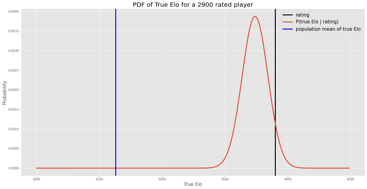
Let’s sanity check this. The mean of the true Elo is a lot lower than 2900, which makes sense since true Elos are much more likely to be lower than 2900 in the “population”. The stdev is smaller than our initial stdev for true Elo (290), which makes sense since we’ve learned something by observing the rating. It’s also smaller than the noise in our observation (110) which honestly surprises me a little1, but I’ve attempted to verify this with simulations and it seems to check out.
Back to business
Let’s take 2 players with a rating difference of 525. Say their respective ratings are 1500 and 2025. We now can compute the PDF of true Elo for each player:
\[\begin{align} \textrm{PDF(true Elo difference | rating = 1500)} \sim \mathcal{N}(1515, 104) \\ \textrm{PDF(true Elo difference | rating = 2025)} \sim \mathcal{N}(1981, 104) \end{align}\]And to compute the PDF of the true Elo difference, we just need to subtract the two normal distributions, which we also know how to do in close form:
\[\textrm{PDF(true Elo difference)} \sim \mathcal{N}(466, 146)\]Last, but not least, we can compute the weighted average (integral) of the Elo formula given this PDF:
\[\begin{align} f(\textrm{Elo difference}) = \frac{1}{1 + 10^{\textrm{(-Elo difference)}/400}} \\ p(x) = \frac{1}{146\sqrt{2\pi}} e^{-\frac{1}{2}\left(\frac{x-466}{146}\right)^{\!2}\,} \\ \int f(x) p(x) dx \approx 0.917 \end{align}\]Close enough?
-
Having dug into this a bit, I now realize that the posterior stdev is always smaller than both the prior stdev and the observation stdev. One way to think about this is that the formulas don’t really care which is the prior and which is the observation - it’s symmetric. So, if it makes sense to me that the posterior stdev should be saller than the prior stdev, then I can mentally use the same reasoning for the observation stdev. ↩