Noisy Elo

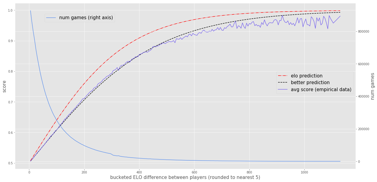
\[\newcommand{\E}{\mathbb{E}} \newcommand{\Ehat}{\hat{\E}} \newcommand{\EElo}{\E_{Elo}} \newcommand{\P}{\mathbb{P}} \newcommand{\Phat}{\hat{\P}}\]

I was chatting with a couple of people about the result of my last post, specifically that the Elo formula systematically overpredicts the expected score of the better player, and one of them had the following neat idea:

What if the Elo formula assumes that the inputs are the true Elo rating of each player (in some sense¹), whereas current Elo ratings are just a noisy measurement of that? By giving the Elo formula a noisy version of the input that it expects, you’d expect to see the empirical results underperform the formula’s prediction.

To understand why, let’s consider an extreme case. Let’s say I told you that the rating of one player was 1,000 points higher than the other, but that the standard deviation of the noise in the Elo ratings was 1,000,000. A true Elo difference of 1,000 points indicates that one player is much better than the other and is almost surely going to win. Accordingly, the Elo formula will predict an expected score of about 1. But if ratings have a stdev of 1,000,000 around the true Elo, a rating difference of 1,000 actually gives you very little information about who is the better player - it’s probably close to 50/50, in which case you’d expect the expected score of the higher rated player to be much lower than 1 (probably about 0.5).

I thought this was a great idea, so I decided to run with it.

Conjecture: Current Elo ratings are a (normally distributed) noisy measurement of true Elo ratings. The empirical expected score of the better player underperforms the Elo formula’s prediction due to this noise.

Let’s start formalizing these ideas with ~~some~~ a lot of notation. You’re probably familiar with some of these symbols already, but just in case:

\[\begin{align*} e_A &: \text{The true Elo rating of player A} \\ r_A &: \text{The current Elo rating of player A} \\ s_A &: \text{The score of player A} \\ \sigma_R &: \text{The stdev of the noise in the current Elo rating} \\ & \text{ (assumed to be normally distributed with mean zero, also assumed to be the same for everyone) } \\ \P[X] &: \text{The probability distribution function of the random variable X} \\ \P[X | Y] &: \text{The PDF of the r.v. X given Y} \\ \E[X] &: \text{The expected value of the r.v. X} \\ \Ehat[X] &: \text{The empirical expected value of the r.v. X} \\ \EElo &: \text{The expected value, assuming the Elo formula} \\ X \sim \mathcal{N}( \mu,\sigma) &: \text{The r.v. X is normally distributed with mean $\mu$ and stdev $\sigma$}\\ \end{align*}\]

So, let’s rewrite our conjecture using these symbols:

Current Elo ratings are a noisy measurement of true Elo ratings. We’re assuming the noise is unbiased (i.e. $\E[r] = e$) and is normally distributed with some standard deviation, $\sigma_R$, which we haven’t specified.

\[\P[ r|e,\sigma _{R}] \sim \mathcal{N}( e,\sigma _{R}) \tag{1}\label{eq:1}\]

The empirical expected score of the better player underperforms the Elo formula’s prediction due to this noise.

\[\Ehat[ s_{A} |r_A,r_B] \approx \E[ s_{A} |r_{A} ,r_{B} ,\sigma _{R}] < \EElo[ s_{A} |r_{A} ,r_{B}] \tag{2}\label{eq:2}\]

Question: What value of $\sigma_R$ best fits the empirical data ($\Ehat[ s_{A} \vert r_A,r_B]$)?

So what is $\E[ s_{A} \vert r_{A} ,r_{B} ,\sigma _{R}]$? This may seem like a big jump, but:

\[\E[ s_{A} |r_{A} ,r_{B} ,\sigma _{R}] =\int\limits_{e_{A}}\int\limits_{e_{B}}\EElo[ s_{A} |e_{A} ,e_{B}] \P[ e_{A} |r_{A} ,\sigma _{R}] \P[ e_{B} |r_{B} ,\sigma _{R}] \mathrm{d} e_{A}\mathrm{d} e_{B} \tag{3}\label{eq:3}\]

In words: for all possible values of $e_A$ and $e_B$, it’s the Elo formula’s prediction of the expected score given those two true Elo ratings, times the probability that those are the true Elo ratings given the current Elo ratings ($r_A$ and $r_B$). In other words, it’s just a weighted average of the Elo formula’s prediction.

Let’s try to define the terms in the double integral. The first one is easy, it’s just the Elo formula (which you can find on wikipedia, although it uses different notation than mine):

\[\EElo[ s_{A} |e_{A} ,e_{B}] =\frac{1}{1+10^{\frac{e_{B} -e_{A}}{400}}}\]

How about the other two terms? The ones of the form $\P[ e \vert r,\sigma_R]$. Let’s use Bayes’ Theorem:

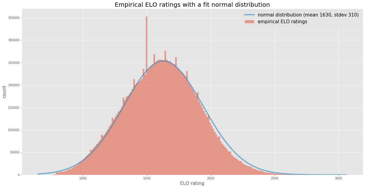
\[\P[ e|r,\sigma _{R}] =\frac{\P[ r|e,\sigma _{R}] \P[ e|\sigma _{R}]}{\P[ r|\sigma _{R}]} \tag{4}\label{eq:4}\]

Now we need to define the three terms that Bayes’ Theorem introduced. The first one ($\P[ r \vert e,\sigma _{R}]$) we already defined from eq $\ref{eq:1}$. The denominator ($\P[ r \vert \sigma _{R}]$) is really just an empirical question: what is the probability distribution function over current Elo ratings? Lucky for you, I came with data. As I explained in my last post, I recently came across an amazing open data set for chess. So, I took a sample of about 10 million games and plotted a histogram of the current Elo ratings, along with a normal distribution that seemed to fit the data pretty well. Take a look:

So, now we can use the following for the denominator:

\[\P[ r | \sigma_R] = \Phat[r] \sim \mathcal{N}( 1630,310) \tag{5}\label{eq:5}\]

Side note: what’s that big spike at 1500? You guessed it - for new players that’s the Elo that this site guesses. So, everyone’s first game has an Elo of 1500. What are those other (smaller) spikes every 50 or so points? Not sure, but my guess is that those are the Elos that are $n$ wins or losses away from 1500, for small values of $n$.

That leaves us with only one more term to define from eq $\ref{eq:4}$: $\P[ e \vert \sigma _{R}]$. Luckily, we’re dealing with normal distributions, which are easy to add and subtract since means and variances are additive.

\[\begin{align*} \P[ r| \sigma _{R}] &= \P[ e \vert \sigma _{R}] + \mathcal{N}( 0, \sigma_R ) \tag{from \ref{eq:1}}\\ \mathcal{N}( 1630,310) &= \P[ e \vert \sigma _{R}] + \mathcal{N}( 0, \sigma_R ) \tag{from \ref{eq:5}} \\ \P[ e \vert \sigma _{R}] &= \mathcal{N}( 1630, \sqrt{310^2 - \sigma_R^2} ) ) \end{align*}\]

We’ve now defined every term in eq $\ref{eq:3}$! That was a lot of symbolic manipulation and not enough graphs. Let’s fix that.

We just defined $\P[ e \vert \sigma _{R}]$, so let’s plot that for a few different values of $\sigma_R$, along with $\Phat[r]$:

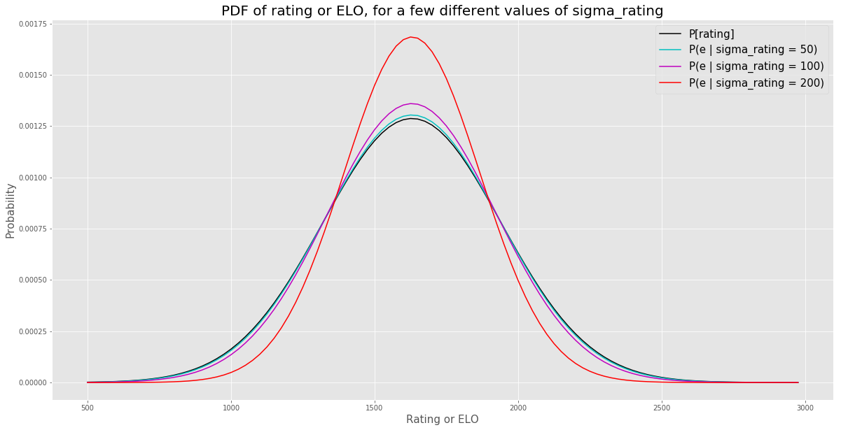
You can see that, as $\sigma_R$ increases, the implied true Elo PDF gets tighter and tigher. Since the variance of the rating PDF is fixed, as we increase the portion of the rating PDF variance that comes from the noise ($\sigma_R^2$), we’re decreasing the amount of variance that comes from the true Elo PDF. For low values of $\sigma_R$, the Elo PDF and the rating PDF look very similar. For higher values of $\sigma_R$, the Elo PDF becomes more concentrated around the mean than the rating PDF. At the extreme, if $\sigma_R$ approaches $310$, the stdev of the rating PDF, the variance of the Elo PDF will go to zero and will become a spike/delta-function/point-mass at the mean of the distribution.

We defined $\P[ e \vert r,\sigma _{R}]$ in eq $\ref{eq:4}$. Let’s see that in action. Let’s plot the Elo PDF conditioned on a given rating, $r = 2800$, for a few different values of $\sigma_R$.

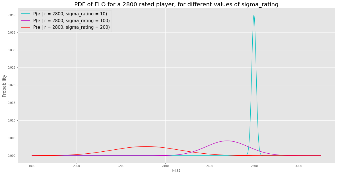
The larger the $\sigma_R$, the more spread out the PDF of Elo is. No surprise there. But the mean decreases as well. Why is that? Well, if the vast majority of people have a true Elo rating under 2500, and I tell you that the current Elo rating is a very noisy measurement of true Elo, doesn’t it make sense to infer that a rating of 2800 is probably a decent amount of positive noise around a much lower true Elo?

That gives me another idea. Let’s plot $\E[ e \vert r, \sigma_R]$ vs. $\sigma_R$ for a few values of $r$:

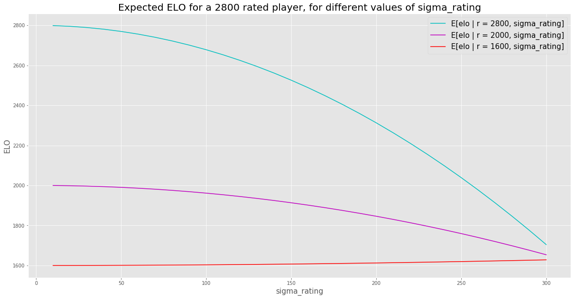
Very cool. If $\sigma_R$ is low, you trust that the true Elo is close to the rating. But as $\sigma_R$ goes up, you’re influenced more and more by the prior that most people’s true Elo is close to the mean of 1630.

All that seems pretty sensible, so let’s see if we can go back and answer our original question. I’ll restate it here: What value of $\sigma_R$ best fits the empirical data ($\Ehat[ s_{A} \vert r_A,r_B]$)?

In case you didn’t read the last post, here is the empirical data to which I’m referring with the term $\Ehat[ s_{A} \vert r_A,r_B]$:

\[\Ehat[ s_{A} | r_A, r_B] \approx \frac{1}{1+10^{\frac{r_B - r_A}{525}}}\]

I’d like to plot $\E[ s_{A} \vert r_{A} ,r_{B} ,\sigma _{R}]$ for a few values of $\sigma_R$ and see which looks closest to $\Ehat$, but we have a little problem. Before, $\E[s]$ only depended on the difference in the two ratings; it didn’t depend on the absolute values of those ratings. However, with my new formula for $\E[ s_{A} \vert r_{A} ,r_{B} ,\sigma_R]$, that’s no longer the case². So what can we do?

Let’s define the rating difference: $\Delta _{AB} =r_{A} -r_{B}$. I think we can construct a new formula for $\E[s]$ as follows:

\[\E[ s_{A} |\Delta _{AB} ,\sigma _{R}] = \int\limits_{r_A} \E[ s_{A} | r_{A} ,r_{B} =r_{A} -\Delta _{AB} ,\sigma _{R}] \P[r_A | \sigma_R] \mathrm{d} r_{A}\]

Basically, for any given $\Delta_{AB}$, we’re taking a weighted average of all the expected scores with that rating difference. Now we can plot $\Ehat$ along with $\E[ s_{A} |\Delta _{AB} ,\sigma _{R}]$ for a few values of $\sigma_R$ and see which looks best:

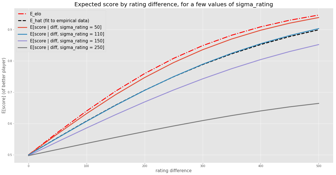
It looks like the blue line, where $\sigma_R = 110$, is an almost perfect match to $\Ehat$. When $\sigma_R$ is lower, like 50, the expected scores are much too high (although still lower than $\EElo$, as you’d expect). When $\sigma_R$ increases to values larger than 110, like 150 and 250, the expected scores are even lower than the observed scores.

And we have our answer. Assuming our conjecture is true, the data suggests that Elo ratings have a standard deviation of about 110 around a player’s true Elo. That’s quite a bit of noise - more than I would have guessed. Actually, I did guess, and my guess was 40. So 110 is a bit of a surprise to me.

Discussion

I’d like to reflect on what we’ve done. We put forth a conjecture about what might explain the underperformance of actual expected scores relative to the Elo formula’s prediction, however our conjecture had a degree of freedom - namely $\sigma_R$. More specifically, we proposed that a player’s Elo rating is normally distributed with a mean equal to the player’s true Elo rating, but we did not specify the standard deviation of that normal distribution. So, we tested several values of $\sigma_R$ against the empirical data to see which $\sigma_R$ looked best.

What can we say about the truth or falsity of our conjecture? Well, we certainly haven’t proven it false. We did find a value for $\sigma_R$ that fit the data well ($\sigma_R = 110$). To be clear, that wasn’t a foregone conclusion. It could have been the case that no $\sigma_R$ looked similar to $\Ehat$. For example, our conjecture could have produced curves that had completely different shapes than $\Ehat$.

But we do have to admit that, given the degree of freedom, it’s not that surprising that we found a $\sigma_R$ that looked pretty good. So we haven’t made that much progress towards proving that our conjecture is likely true³. How can we proceed?

Well, recently I’ve been reading about the history of progress in physics, and this situation looks kind of familiar. You have a theory for how the world works, but new empirical data shows up that disagrees with the theory. Assuming the new data is valid, you try to come up with a new model that fits the data. And you find one! Your model fits the new data well. But how do you convince others to use your new model, especially in light of potentially other new models that also fit the data? One approach is to propose a new experiment for which your model predicts a different outcome than the old model. If your model predicts the correct outcome of a yet-to-be-conducted experiment, for which the old model would have been wrong, that’s fairly compelling evidence to start using it in place of the old model.

Can we do that here? I think the answer is yes, but this post is already pretty long and dense, so let’s leave that for a future post.

What do I mean by true Elo rating? I’m not totally sure, but maybe something like: the expected rating of a player in the limit of them playing infinity games (without actually getting better though, which would increase their true Elo). ↩
I later realized that the new formula also only depends on the rating difference, but that’s not obvious from the formula itself. ↩
I understand that you can never actually prove it to be true. ↩