The Two Envelopes Problem
If you haven’t already encountered the famous paradoxical “two envelopes problem”, then I highly suggest you consider the following prompt and return to this article much later. Without struggling with the problem yourself first, the “resolution” below won’t seem nearly as satisfying.
From Wikipedia:
You are given two indistinguishable envelopes, each containing money. One contains twice as much as the other. You may pick one envelope and keep the money it contains. Having chosen an envelope at will, but before inspecting it, you are given the chance to switch envelopes. Should you switch?
It seems that you can make compelling arguments for “always switch” and “it doesn’t matter whether or not you switch”.
Always switch: Let’s denote the amount of money in the envelope that you chose as \(X\). The other envelope contains either \(2X\) or \(\frac{1}{2}X\). If we think these outcomes are equally likely, then the expected value of switching is \(\frac{1}{2}(2X) + \frac{1}{2}(\frac{1}{2}X) = \frac{5}{4}X\). In other words, if you switch then, in expectancy, you end up with more than you started. So always switch!
It doesn’t matter: But that seems crazy! The problem is completely symmetric: you’re presented with two envelopes and you chose one at random. Why would it make any sense to switch when you could have just as easily randomly chosen the other envelope? Furthermore, if you do switch and then are presented with the option to switch again, doesn’t the same logic apply? But switching twice is the same as not switching so… that can’t be right. Common sense (and symmetry) strongly suggests that switching can’t matter.
One common objection to the argument for always switch above is that we assumed that getting \(\frac{1}{2}X\) and \(2X\) were equally likely, but that doesn’t make a lot of sense. If the probability of the other enveloping having \(\frac{1}{2}X\) or \(2X\) were the same, that implies the following two states are equally likely: the two envelopes have \(\frac{1}{2}X\) and \(X\) in them, or the two envelopes have \(X\) and \(2X\) in them. We will denote these pairs of amounts as \((\frac{1}{2}X, X)\) and \((X, 2X)\).
But then we can apply the same logic to the case where our chosen envelope has \(2X\) in it and we conclude that the pairs \((X, 2X)\) and \((2X, 4X)\) must also be equally likely. And so on for \((2X, 4X)\) and \((4X, 8X)\), \((4X, 8X)\) and \((8X, 16X)\), and so on. We can also apply this logic to smaller and smaller pairs of amounts, e.g. \((\frac{1}{4}X, \frac{1}{2}X)\) and \((\frac{1}{2}X, X)\), \((\frac{1}{8}X, \frac{1}{4}X)\) and \((\frac{1}{4}X, \frac{1}{2}X)\), etc. In effect, you end up with an infinite number of equally likely possibilities, which is an improper prior distribution. We need the sum of the probabilities of our possible pairs of amounts to equal \(1\), but when we sum the probabilities of this weird improper distribution, we effectively get \(\infty \cdot \frac{1}{\infty}\), which is not well defined.
Furthermore, the problem didn’t actually say that getting \(\frac{1}{2}X\) and \(2X\) were equally likely, so let’s dispense with that assumption.
To make this discussion more rigorous and less vague, let’s consider a new problem that has the same paradoxical properties as the origional one, but in which we know the exact distribution of the outcomes. To give credit where credit is due, everything below is due to the following excellent youtube video: https://www.youtube.com/watch?v=_NGPncypY68.
A more well-specified problem
Below is a table of all possible states that the two envelopes (A and B) can be in, along with the probability of being in that state:
| State | Probability | Envelope A | Envelope B |
|---|---|---|---|
| \(S_1\) | 1/2 | $1 | $10 |
| \(S_2\) | 1/4 | $10 | $100 |
| \(S_3\) | 1/8 | $100 | $1,000 |
| … | |||
| \(S_n\) | \(1/2^n\) | \(10^{n-1}\) | \(10^n\) |
To be clear, there are infinitely many states (not just \(n\) of them). Given that, the probabilities sum to \(1\), as they should. As in the original problem, you choose an envelope at random - meaning you’ll choose Envelope A with a 50% chance and Envelope B with a 50% chance, but you won’t know which one you’ve chosen. After picking an envelope, but before inspecting it, you’re given the option to switch. Should you?
To decide whether or not we should switch envelopes, let’s compute the expected value of switching. I’m going to use the “law of total expectation”, which is a fancy way of saying that I’ll compute \(E[switching]\) by:
\[E[switching] = \sum\limits_{Y=y} E[switching | Y = y] \cdot P[Y = y]\]Where \(Y\) is some other random variable. I’m not saying concretely what \(Y\) is because I’m going to compute this three different ways using three different \(Y\)s.
1. \(Y\) is which state we’re in (\(S_1\), \(S_2\), \(S_3\), … )
To start, let’s compute the E[switching] by conditioning on which state we’re in.
\[\begin{align} E[switching] &= E[switching | state = S_1] \cdot P[state = S_1] \\ &+ E[switching | state = S_2] \cdot P[state = S_2] \\ &+ E[switching | state = S_3] \cdot P[state = S_3] \\ ... \end{align}\]Now we just need to compute each term:
\[\begin{align} E[switching | state = S_1] &= 1/2 (+9) + 1/2 (-9) &= 0 \\ E[switching | state = S_2] &= 1/2 (+90) + 1/2 (-90) &= 0 \\ E[switching | state = S_3] &= 1/2 (+900) + 1/2 (-900) &= 0 \\ \end{align}\]… you get the picture. Every term = 0, so E[switching] is clearly = 0.
2. \(Y\) is the value in the envelope we picked
We’ll do exactly what we did before, but instead of conditioning on which state we’re in, let’s condition on the value of the envelope we picked (note: we don’t know this value, but it must have some value, right?):
\[\begin{align} E[switching] &= E[switching | picked = \$1] \cdot P[picked = \$1] \\ &+ E[switching | picked = \$10] \cdot P[picked = \$10] \\ &+ E[switching | picked = \$100] \cdot P[picked = \$100] \\ ... \end{align}\]Now we compute the terms:
\[\begin{align} E[switching | picked = \$1] &= +9 &> 0 \\ E[switching | picked = \$10] &= 2/3 (-9) + 1/3 (+90) &> 0 \\ E[switching | picked = \$100] &= 2/3 (-90) + 1/3 (+900) &> 0 \\ \end{align}\]… you get the picture. Every term > 0 (and we multiply each term by some positive probability), so E[switching] is clearly > 0.
3. \(Y\) is the value in the other envelope
We’ll do exactly what we did before, but instead of conditioning on the value in the envelope that we picked, we’ll condition on the value of the envelope we didn’t pick (which I’m calling “other”):
\[\begin{align} E[switching] &= E[switching | other = \$1] \cdot P[other = \$1] \\ &+ E[switching | other = \$10] \cdot P[other = \$10] \\ &+ E[switching | other = \$100] \cdot P[other = \$100] \\ ... \end{align}\]Now we compute the terms:
\[\begin{align} E[switching | other = \$1] &= -9 &< 0 \\ E[switching | other = \$10] &= 2/3 (+9) + 1/3 (-90) &< 0 \\ E[switching | other = \$100] &= 2/3 (+90) + 1/3 (-900) &< 0 \\ \end{align}\]… you get the picture. Every term < 0 (and we multiply each term by some positive probability), so E[switching] is clearly < 0.
What gives!?
According to the video (and I don’t know how much I should trust this random video), here’s what gives: The random variable “profit of switching envelopes” has no expected value. It’s not zero, it’s not positive infinity, and it’s not negative infinity. It’s simply not defined. This also explains why using the “law of total expectation” breaks down. As the Wikipedia article states, you can only use the law of total expectation on a random variable \(X\) if \(E[X]\) is defined. Here is a link to the video at the moment that he explains the resolution: https://youtu.be/_NGPncypY68?t=1213
When we compute the expected value, we’re summing up an infinite number of terms. In this case, the order in which we sum the terms matters. This is a very unusual property. This property occurs when the sum of all the positive terms in the series is +infinity and the sum of all the negative terms is -infinity. In those cases, you can rearrange the order of summation and get completely different results. Since no one summation order is “more correct” than another, this infinite series has no well-defined sum.
In case it’s not obvious, notice that in the three versions of E[switching] above, the only difference is the way in which we ordered and then grouped the terms of the sum. Here’s a picture to make it more clear:
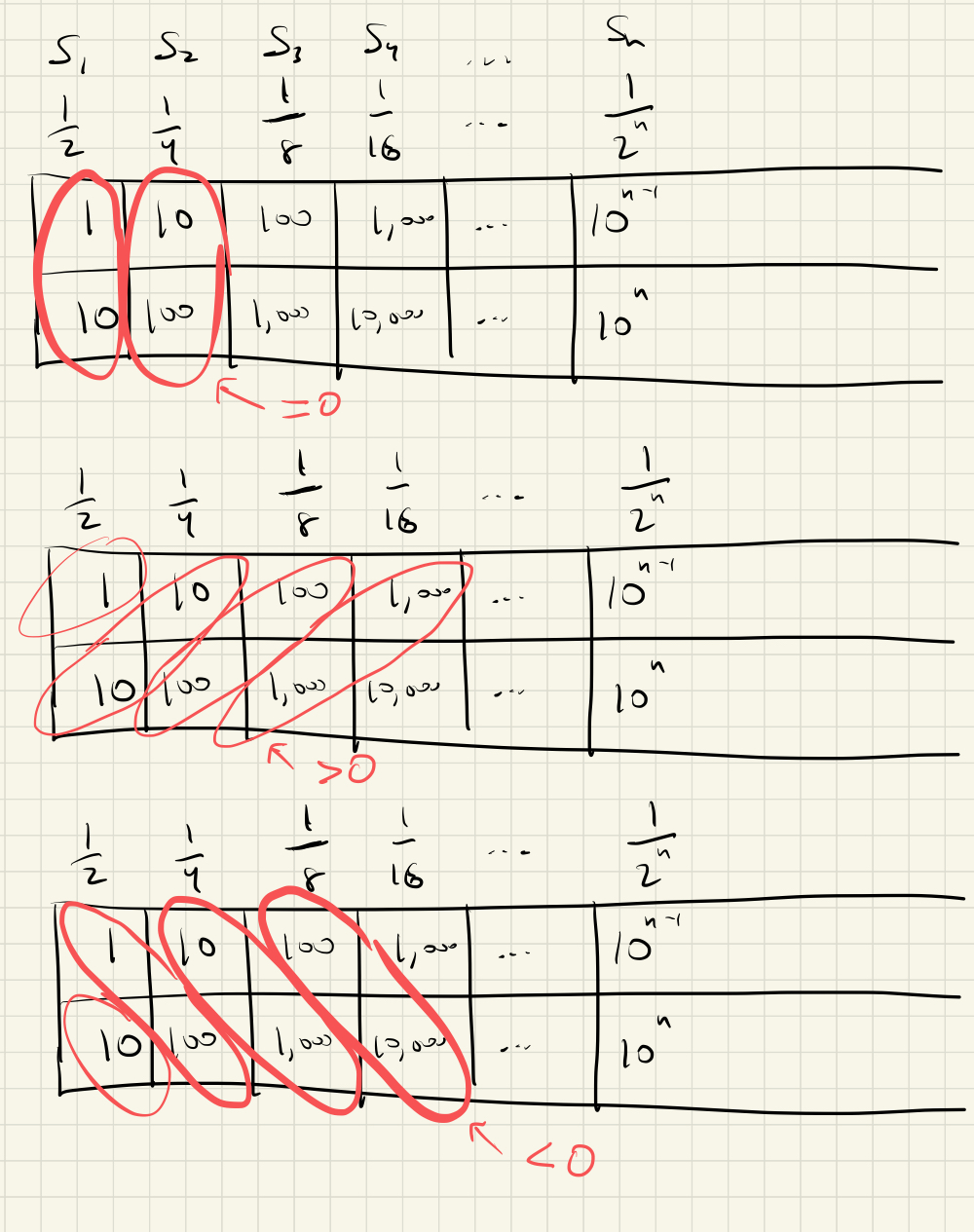
The thing I like about this explanation is that it not only resolves the paradox, but it also shows why you can make convincing arguments for either strategy (switch or don’t switch).
Remaining dissonance
Although I’m quite pleased with the resolution above, I’m still a bit unsettled by the fact that I would still answer “yes” to the following two questions:
If we changed the “well-specified problem” to say that you could open the envelope you chose before deciding whether or not to switch, would you conclude that switching is better no matter what you saw in your envelope?
If we changed the “well-specified problem” to say that you could open the other envelope before deciding whether or not to switch, would you conclude that switching is worse no matter what you saw in your envelope?