G11. Primitive Recursive Functions
Godel’s incompleteness theorem talks about formal systems that are “sufficiently strong”. In this post, we will clarify what exactly is meant by that phrase.
Primitive recursive functions are a very large class of functions that, very roughly speaking, correspond to functions that you can compute “with only for loops”. The constraint of using only for loops (as opposed to while loops) means that these functions cannot create infinite loops and will therefore always complete in a finite number of steps. Furthermore, the number of steps it will take to complete is bounded (since for loops have a predetermined length). We will define them much more precisely later, but first we should talk about why we’re interested in them.
Motivation
As we mentioned in the previous post, Godel defined what is known as “the Godel sentence” which can be interpreted as “this statement cannot be derived within this formal system”. At first glance, it’s not obvious that such a statement can be constructed within the formal system that Godel was using. However, Godel meticulously built up a series of relations - helper functions if you will - that he used in building his sentence. Furthermore, he showed that each one is “primitive recursive”. Lastly, he showed that his formal system can express (actually capture) any primitive recursive relation. Through this chain of logic, he showed that his formal system can express the Godel sentence.
This chain of logic actually says a bit more. It shows that any formal system, not just the one that Godel was using, that can express all primitive recursive relations can express a version of “the Godel sentence”. This is what is meant by a sufficiently expressive formal system: a formal system that can express all primitive recursive relations. The stronger version of this is a sufficiently strong formal system, which is a formal system that can capture all primitive recursive relations.
Remember that expressing a relation between two numbers \(x\) and \(y\) with an open formula \(\varphi(x, y)\) means that the formula is true iff \(x\) and \(y\) have that particular relation, while capturing the relation means that \(\varphi(x, y)\) is derivable within the formal system if \(x\) and \(y\) have that particular relation and \(\lnot \varphi(x, y)\) is derivable if not.
Expressing is to truth as capturing is to derivability.
Hopefully that sufficiently motivates the desire to understand what a primitive recursive relation (or function) actually is. So let’s get started.
Definition
As with all of my posts, there probably exist better explanations out there on the internet. In this case, however, I think I’ve found one. The first 4 videos of this 5-video YouTube playlist do an excellent job at defining and explaining primitive recursive functions. I will attempt to explain it myself below, but I highly recommend watching those videos.
We will start with the precise, but incredibly abstract definition and then work through a series of examples.
A quick note about notation before we start. Functions that take \(n\) arguments are called \(n\)-ary functions. One notational method to make it clear that a function takes \(n\) arguments to write it like so \(f(x_1, \ldots, x_n)\). This is clear and intuitive, but long - especially when composing \(k\) functions each with \(m\) arguments. A different method would be to notate each \(n\)-ary function with an \(n\) superscript, like so: \(f^n\). We will use both methods below.
The basic primitive recursive functions are given by these axioms:
- Constant function: The 0-ary constant function \(Z^0 = 0\) is primitive recursive.
- Successor function: The 1-ary successor function \(S^1\), which returns the successor of its argument, is primitive recursive. That is, \(S^1(k) = k + 1\).
- Projection function: For every \(n≥1\) and each \(i\) with \(1≤i≤n\), the \(n\)-ary projection function \(P^n_i\), which returns its \(i\)-th argument, is primitive recursive. For example, \(P^3_2(x,y,z) = y\).
More complex primitive recursive functions can be obtained by applying the operations given by these axioms:
-
Composition: Given a \(k\)-ary primitive recursive function \(f^k\), and \(k\) many \(m\)-ary primitive recursive functions \(g^m_1,\ldots,g^m_k\), the composition of \(f^k\) with \(g^m_1,\ldots,g^m_k\), i.e. the \(m\)-ary function \(h^m(x_1,\ldots,x_m) = f^k(g^m_1(x_1,\ldots,x_m),\ldots,g^m_k(x_1,\ldots,x_m))\) is primitive recursive.
-
Primitive recursion operator: Given \(f^k\), a \(k\)-ary primitive recursive function, and \(g^{k+2}\), a \((k+2)\)-ary primitive recursive function, the primitive recursion of \(f^k\) and \(g^{k+2}\) is defined as the \((k+1)\)-ary function \(h^{k+1}\) constructed as follows: \(\begin{aligned} h^{k+1} (0, x_1, \ldots, x_k) &= f^k (x_1, \ldots, x_k) \\ h^{k+1} (S(y), x_1, \ldots, x_k) &= g^{k+2} (y, h (y, x_1, \ldots, x_k), x_1, \ldots, x_k)\end{aligned}\)
We will use the symbol \(Pr^{k+1}(f^k,g^{k+2})\) to indicate the primitive recursion of \(f^k\) and \(g^{k+2}\).
The primitive recursive functions are the basic functions and those obtained from the basic functions by applying composition and primitive recursion a finite number of times.
Interpretation of the Primitive Recursion Operator
In a rare turn of events, Wikipedia gives a (somewhat) intuitive way to think about the primitive recursive operator as a for loop:
Interpretation. The function \(h\) acts as a for loop from 0 up to the value of its first argument. The rest of the arguments for \(h\), denoted here with \(x_i\)’s \((i = 1, \ldots, k)\), are a set of initial conditions for the for loop which may be used by it during calculations but which are immutable by it. The functions \(f\) and \(g\) on the right side of the equations which define \(h\) represent the body of the loop, which performs calculations. Function \(f\) is only used once to perform initial calculations. Calculations for subsequent steps of the loop are performed by \(g\). The first parameter of \(g\) is the “current” value of the for loop’s index. The second parameter of \(g\) is the result of the for loop’s previous calculations, from previous steps. The rest of the parameters for \(g\) are those immutable initial conditions for the for loop mentioned earlier. They may be used by \(g\) to perform calculations but they will not themselves be altered by \(g\).
Examples
The only way that I was able to really understand primitive recursion was seeing many examples and then working through a few myself. Let’s start with an easy one.
Add2(x) = x + 2
To implement \(Add2^1(x) = x + 2\), we just need to apply the successor function \(S^1\) twice, which we can do via composition. Since the successor function is primitive recursive and composition is also primitive recursive, then the resulting \(Add2^1\) function is also primitive recursive.
\(Add2^1(x) = S^1(S^1(x)) = x + 2\)
Zero(x) = 0
Notice that the 0-ary zero function \(Z^0\) is given to us as an axiom, but not the 1-ary zero function \(Z^1(x) = 0\). We can define it ourselves using primitive recursion:
\(\begin{aligned} Z^1(0) &= f^0() = Z^0 \\ Z^1(y+1) &= g^2(y, Z^1(y)) = P^2_2(y,Z^1(y)) = Z^1(y) \\ Z^1 &= Pr(f^0, g^2) \end{aligned}\)
Try to manually compute \(Z^1(2)\) using the definition above. Once you’re done, click here to check your work.
Add(x,y) = x + y
\(\begin{aligned} Add^2(0, y) &= f^1(y) = P^1_1(y) = y \\ Add^2(x+1, y) &= g^3(x, Add^2(x,y), y) = S(P^3_2) = Add^2(x,y) + 1 = x + y + 1 \\ Add^2 &= Pr(f^1, g^3) \end{aligned}\)
Mult(x,y) = x * y
\(\begin{aligned} Mult^2(0, y) &= f^1(y) = Z^1(y) = 0 \\ Mult^2(x+1, y) & = g^3(x,Mult(x,y), y) = Add^2(P^3_2, P^3_3) = Add^2(Mult(x,y),y) = x \cdot y + y \\ Mult^2 &= Pr(f^1, g^3) \end{aligned}\)
Notice the role of the projection functions in the examples thus far. They serve a critical, but trivial role. They allow you to select which arguments to pass to another function. In \(Add^2\), the composition of \(S(P^3_2)\) is just the function \(g(x,y,z) = S(y)\), since \(P^3_2\) is a function which takes 3 arguments and returns the 2nd. In \(Mult^2\), \(Add^2(P^3_2, P^3_3)\) is really just a confusing way to write \(g(x,y,z) = Add^2(y, z)\). From now on, for the sake of readability, I will omit the projection functions and allow myself to select and reorder arguments with the knowledge that we can make this rigorous via the use of projection functions if we need.
Also notice that I used \(Add^2\) to define \(Mult^2\). This is perfectly acceptable since primitive recursive functions are the basic functions and those obtained from the basic functions by applying composition and primitive recursion a finite number of times. So, we can use any primitive recursive function in the definition of another primitive recursive function.
Practice is critical in order to intuitively grasp how primitive recursion is like a for loop. Try to manually compute \(Mult^2(3,5)\). Once you’re done, click here to check your work.
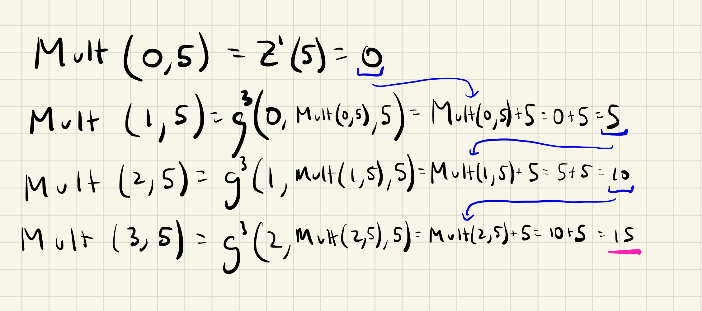
Pow(n, x) = \(x^n\)
\(\begin{aligned} Pow^2(0, x) &= f^1(x) = S(x) \\ Pow^2(n+1, x) &= g^3(n, Pow^2(n, x), x) = Mult^2(x, Pow^2(n,x)) = x \cdot x^n \\ Pow^2 &= Pr(f^1, g^3) \end{aligned}\)
Are you getting the hang of these yet? If you can define a base case for when the first argument is equal to 0, and a recursive case that computes \(f(x+1,y)\) based on some combination of \(x\), \(y\), and \(f(x,y)\), then you can combine these using primitive recursion to define your function for any \(x\) and \(y\).
A Goal: The Div function
We’re going to now head towards an ambitious goal. I want to define the following primitive recursive function: \(Div(x,y)\) which equals \(1\) if \(x\) is divisible by \(y\) and \(0\) otherwise. To do this, we’re going to need to build up a series of simpler primitive recursive functions to help.
Sgn(x) = 1 if x > 0 else 0
\(\begin{aligned} Sgn^1(0) &= f^0() = Z^0 = 0 \\ Sgn^1(x+1) &= g^2(x, Sgn(x)) = S(Z^2) = 1 \\ Sgn^1 &= Pr(f^0, g^2) \end{aligned}\)
Pred(x) = max(0, x - 1)
Note that our “predecessor” function can never be negative, because primitive recursive functions only deal with the natural numbers, so \(Pred(0) = 0\).
\[\begin{aligned} Pred^1(0) &= f^0() = Z^0 = 0 \\ Pred^1(x+1) &= g^2(x, Pred^1(x)) = x \\ Pred^1 &= Pr(f^0, g^2) \end{aligned}\]Sub(x,y) = max(0, y - x)
Note that our subtraction function can never be negative, like \(Pred\). Also note that \(Sub(x,y)\) is \(max(0, y - x)\) not \(max(0, x - y)\).
\[\begin{aligned} Sub^2(0, y) &= f^1(y) = y \\ Sub^2(x+1, y) &= g^3(x, Sub^2(x,y), y) = Pred^1(Sub^2(x,y)) \\ Sub^2 &= Pr(f^1, g^3) \end{aligned}\]Absdiff(x,y) = \(| x - y|\)
\(Absdiff^2(x,y) = Add^2(Sub^2(x,y),Sub^2(y,x))\)
Neq(x,y) = 1 if \(x \neq y\) else 0
\(Neq^2(x,y) = Sgn^1(Absdiff^2(x,y))\)
Eq(x,y) = 1 if \(x = y\) else 0
\(Eq(x,y) = Sub^2(Neq^2(x,y), S^1(Z^2)) = 1 - Neq^2(x,y)\)
Rem(x,y) = x % y
\[\begin{aligned} Rem^2(0, y) &= f^1(x) = Z^1(x) = 0 \\ Rem^2(x+1, y) &= g^3(x, Rem^2(x, y), y) = Neq(Rem^2(x,y) + 1,y) \cdot (Rem^2(x,y) + 1) \\ Rem^2 &= Pr(f^1, g^3) \end{aligned}\]The recursive case (\(g^3\)) is a little unintuitive. It basically says, if the (remainder of x / y) + 1 = y then 0 else (remainder of x / y) + 1.
Div(x,y) = 1 if x is divisible by y else 0
\[\begin{aligned} Div^2(x,y) = Eq^2(Rem^2(x,y),Z^2(x,y)) = Eq^2(Rem^2(x,y), 0) \end{aligned}\]The last step was refreshingly simple. No primitive recursion, just simple function composition.
What’s not primitive recursive?
When introducing a property, it’s helpful to show a few examples of things that do not have that property. In this case, what functions are not primitive recursive?
Let’s take a step back and define three broad classes of functions:
- Primitive Recursive Functions
- Computable functions that are not primitive recursive
- Uncomputable functions
Intuitively, the primitive recursive functions are the set of functions that can be computed using “only for loops” which means they must terminate (there are no infinite while loops) and the number of steps can be bounded (since for loops have a predetermined length).
What, then, are computable functions? Intuitively, computable functions are the set of functions that can be computed by a computer (e.g. a Turing machine) given unlimited amounts of time and space. Essentially, we remove the restriction that it must only use for loops which means that the number of steps it takes to compute the result is no longer necessarily bounded. The most classic example of such a function is the Ackermann function.
What, then, are the uncomputable functions!? An unhelpful (but accurate) definition is that they are the set of functions that are not… computable. A more intuitive definition is that there is no finite procedure (or algorithm) that can compute the function. The most famous example of such a problem is the Halting problem. A simpler example is the Busy beaver. I will give a slapdash explanation of the busy beaver problem here and why it’s uncomputable.
An “nth Busy beaver” is binary-alphabet Turing machine with \(n\) states that reads a tape initially consisting of all zeros. The Turing machine will run and must eventually halt. At the point of halting, the tape must contain as many or more 1’s on it than any other \(n\) state Turing machine would produce under the same scenario.
The Busy beaver function takes as input \(n\) and returns the number of 1’s that the “nth Busy beaver” would produce. Wikipedia states that determining whether an arbitrary Turing machine is a busy beaver is undecidable.
You may think: why not just enumerate all possible \(n\)-state binary-alphabet Turing machines, run them all, and see which one produces the most 1’s after they all halt? I think the problem with this is that some of those Turing machines may run forever. Consider a Turing machine that you’re attempting to “test” that has run for one millions steps so far. How would you reliably decide whether or not it will eventually halt? This seems like the Halting problem, which is also uncomputable. Take this entire paragraph with a large grain of salt as these are my own speculations and I’m relatively new to these ideas.
One interesting addendum is that most functions are uncomputable, which is unintuitive given every function we run into on a daily basis is probably computable. This reminds me of the fact that almost all real numbers are trancendental, but I bet you can’t name more than 2.