Why correlation is the key to quantum computing
I think most lay articles about quantum computing completely gloss over a critical detail for why the state of quantum computers is exponentially larger than that of classical computers. They reference the probabilistic nature of qubits - the fact that a qubit can be in a superposition of both 0 and 1 - as the property that makes quantum states exponentially large, but that’s only part of the explanation. The other critical property is that the qubits are not independent; they’re correlated with each other. This is often briefly mentioned as quantum entanglement, but rarely explained. Let me give it a shot.
A computer with \(N\) bits can be in one of \(2^N\) states. In this article, we’ll use N = 3 to keep things manageable. Here they are:

How many bits do you need to describe which state the computer is in? 3, obviously. This question feels oddly circular in the case of classical computers since the bits that describe which state you are in are exactly the bits that are in the state itself. This is not true, however, for quantum computers.
A quantum computer with \(N\) qubits can be in a superposition of \(2^N\) states. This is a fancy way of saying that if you observed the state of the computer, there is some probability that you would observe it in any one of the \(2^N\) states. Using N = 3, here’s an example with made up probabilities associated with each state:

You can vary these probabilities by performing operations on the computer. So, if you were to completely describe the state of the computer, you would need to write down the probability1 that it would land in each of the \(2^N\) states. That is… \(2^N\) numbers. Actually, it’s \(2^N - 1\), since the probabilities must sum to 1, so the last number is not “free” in the same way the first \(2^N - 1\) numbers are, but that’s a minor detail. Details aside, this is what people mean when they say that quantum computers contain exponentially more “information” than classical computers. An \(N\)-bit classical computer’s state can be described with \(N\) numbers (bits, actually), while an \(N\)-qubit quantum computer’s state can be described with ~\(2^N\) numbers. That’s a big difference.
But what properties of quantum computers give you this exponential blowup in complexity? Usually, the probabilistic nature of qubits is what gets all the press, but I’m going to show that probabilistic bits by themselves are not sufficient, whereas correlation is.
Consider the example above, with 3 qubits. What is the probability that the first qubit is 0? We can simply add up the probability that the (quantum) computer is in the first four states (000, 001, 010, 011) to get 0.8. What is the probability that the first qubit is 0 conditioned on the second qubit being 0? To compute this, first we eliminate the 4 states where the second qubit is 1, then we compute the probability the the first qubit is 0 and divide by the sum of the remaining 4 probabilities. Here’s a picture:

Notice the probability is still 0.8. It didn’t change. Put into a formula, \(P(q_1 = 0 | q_2 = 0) = P(q_1 = 0) = 0.8\). Put into words, the observation that \(q_1 = 0\) does not depend on - or is independent of - the observation that \(q_2 = 0\).
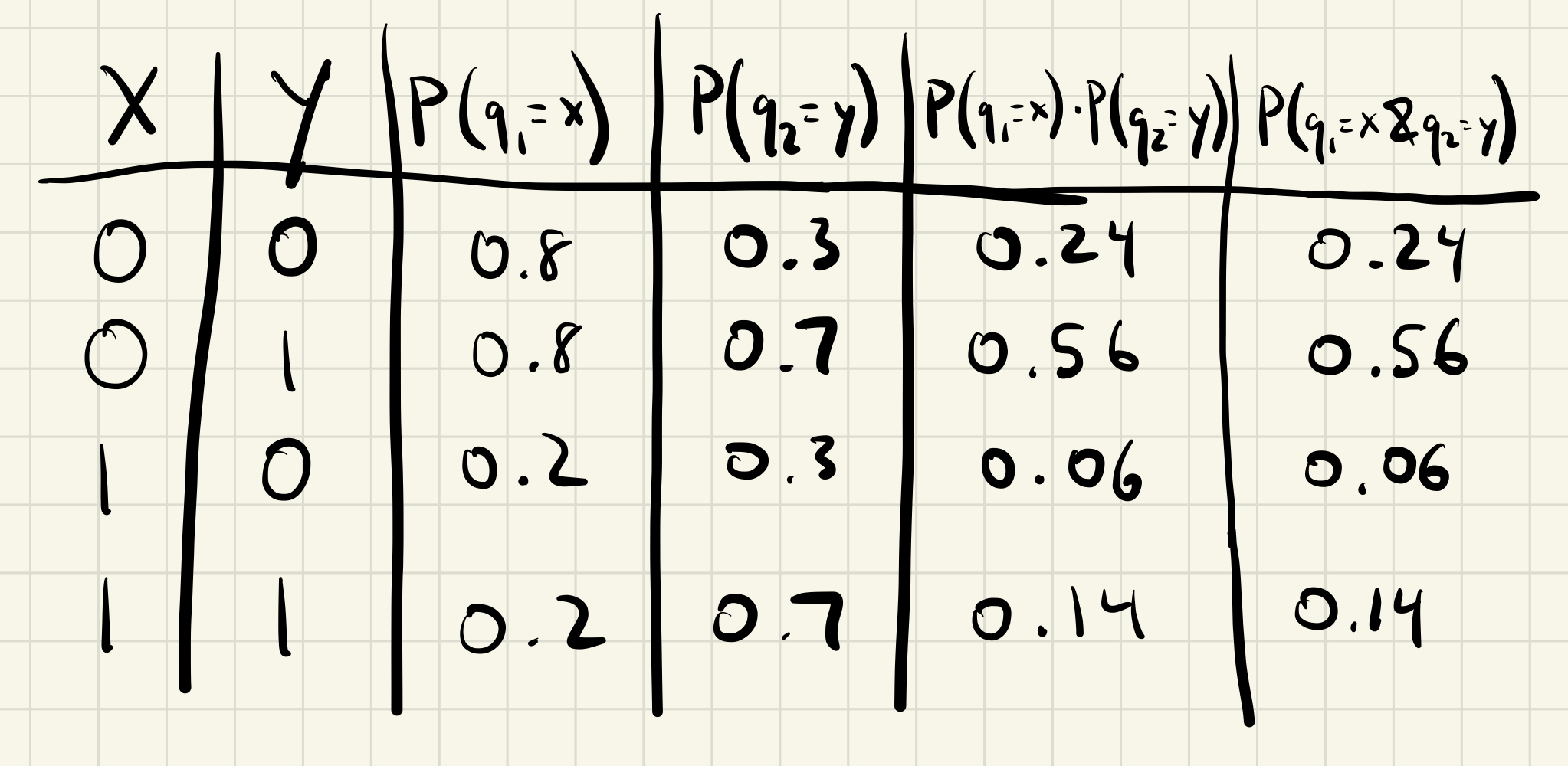
More generally, if the state of \(q_1\) is independent of \(q_2\), then \(P(q_1 = x, q_2 = y) = P(q_1 = x) \cdot P(q_2 = y)\). The following table demonstrates that, with our example probabilities, this is in fact true about qubits \(q_1\) and \(q_2\).
I will leave it as an exercise for the reader to verify that the state of \(q_1\) and \(q_2\) are also independent of \(q_3\). That is, for any state, \(q_1 = x, q_2 = y, q_3 = z\) one can compute the probability of that state by computing \(P(q_1 = x) \cdot P(q_2 = y) \cdot P(q_3 = z)\). To help you out, \(P(q_3 = 1) = 0.9\).
Why is this so important? It’s precisely this property of independent events that allows you to compute the probability of any one of the 8 possibilities (or \(2^N\) more generally) with only 3 numbers (or \(N\) more generally). By knowing the 3 numbers \(P(q_1 = 1)\) and \(P(q_2 = 1)\) and \(P(q_3 = 1)\), you can compute the probability of any one of the 8 possible \([q_1, q_2, q_3]\) states. Remember, the reason that quantum computers contain so much more information than classical computers is because you need ~\(2^N\) numbers to describe their state. But as I’ve just shown, this is not true if the qubits are independent.
A more probabilistic way to state this is that the joint probability distribution of the \(N\) qubits, which is of size \(2^N\), can be factored into the \(N\) marginal distributions of each single qubit, which is of size \(2N\). That sentence contains a lot of jargon that I don’t plan to explain, but if you already have a background in probability theory then it be helpful to you.
So, having probabilistic bits (qubits) by itself does not give you an exponential increase in information. What really matters is that the qubits are not independent, and therefore cannot be factored into a product of the \(N\) single-qubit probability distributions of size 2 (each of which only requires 1 number since if \(P(q = 0) = x\), then \(P(q = 1) = 1 - x\)). If the states of each qubit are correlated (entangled), then it really does require up to \(2^N-1\) numbers to describe the state of an \(N\)-qubit quantum computer, and that’s when the magic happens2.
-
Technically, you’d want the quantum amplitudes associated with each state, not just the probabilities. If the quantum amplitude associated with a given state is \(\alpha\), then the probability of observing the computer in that state is \(\mid \alpha \mid ^2\). ↩
-
Exactly what magic, I don’t know. Something about breaking the entire internet, I think… ↩