Deriving the Taylor Series
My previous post Deriving the Maclaurin Series is a prerequisite for this post.
We’ve just learned how to approximate a function \(f(x)\) using the Maclaurin Series. It’s a pretty sweet hammer, so let’s start hitting some nails. How about \(e^x\)?
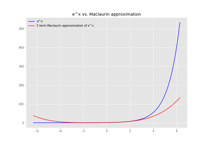
If you care about the region around 0, you’re golden. This is a great approximation. But what if you care about \(x = 6\)? It’s… not great. One option is to add more terms. We used the first 5 terms of the Maclaurin Series. We could use 100. That would definitely work. However, if you know beforehand that you care about a particular region that is not the region around 0, there’s a better way.
When might you know beforehand which x-region you care about in real life? Actually, quite often. Let’s say the function you’re approximating is the percentage humidity in the air as a function of temperature. Are you particularly interested in a temperature of 0? Probably not. You’re probably most interested in temperatures that are close to your current temperature. If you come up with real-life examples, there’s often a natural “default” x value and you probably care most about the x-region around that default value.
So what’s the better way? It’s called the Taylor Series, and it’s just two small steps away from the Maclaurin Series.
Step 1
We want the polynomial \(p\) that best approximates a function \(f\) around the point \(f(a)\). However, as a first step, we’re first going to solve for a polynomial \(p'\) that is almost the polynomial we want. It’s going to be exactly the Maclaurin Series, except in place of \(f(0)\), \(f'(0)\), etc., we’re going to use \(f(a)\), \(f'(a)\), etc. I.e.
\[p'(x) = f(a) + f'(a)x + \frac{f''(a)}{2!}x^2 + \frac{f'''(a)}{3!}x^3 + \dots + \frac{f^{(n)}(a)}{n!}x^n + \ldots\]Because we’re now using the function value (and derivatives) around \(x = a\), the resulting polynomial will look very similar to \(f\) around \(a\). The only problem is that it’s still centered around the origin.
A picture is going to be much easier to understand:
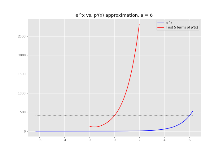
Notice how the red line, \(p'(x)\) has the same value and shape around \(x = 0\) as \(f(x)\) does around \(x = 6\)?
Step 2
This is the easy step, we need to shift our function to the right by \(a\). You may just remember this back from algebra, but if not, we want \(p(x) = p'(x - a)\).
\[\begin{align*} p(x) &= p'(x - a) \\ &= f(a) + f'(a)(x - a) + \frac{f''(a)}{2!}(x - a)^2 + \frac{f'''(a)}{3!}(x - a)^3 + \dots + \frac{f^{(n)}(a)}{n!}(x - a)^n + \ldots \end{align*}\]And, not that it will surprise you, but here’s the final picture (re-centered around \(x = 6\)):
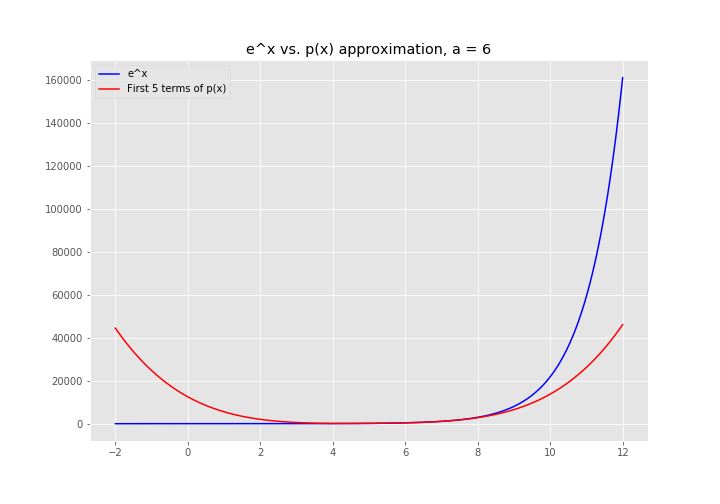
Notice that \(p(x)\) is a much worse approximation of \(e^x\) around \(x = 0\), similar to how the Maclaurin Series was a terrible approximation around \(x = 6\). There’s no magic going on here. We traded off accuracy around \(x=0\) for accuracy around \(x=6\). If you need more accuracy everywhere, you need more terms.